Mistral made four small forecasting models. The baseline still gets a chair

THE SIGNAL IN ONE SENTENCE

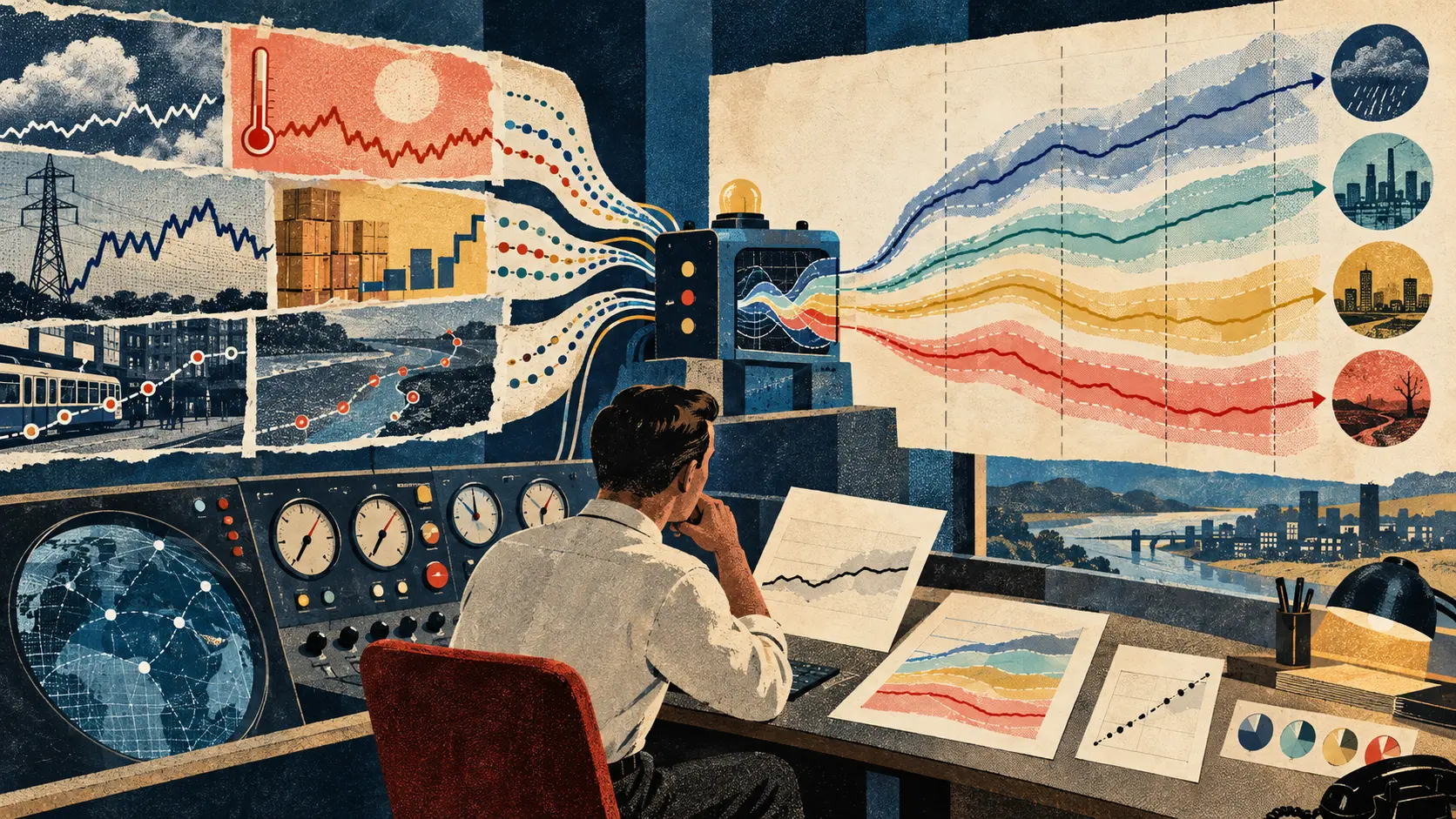
Every company has a time machine. Most of them call it a spreadsheet. Someone takes yesterday's sales, last week's power demand or the last three months of vibration readings and draws a line into tomorrow. The line is useful right up until a holiday arrives, a pump starts behaving strangely or the weather remembers that it has free will. Mistral has released Timestral, a family of four small foundation models built specifically for time-series forecasting. The models range from five million to 209 million parameters. They take historical measurements, related variables and information already known about the future, then return a set of possible outcomes rather than one heroic guess. The largest model is 837 megabytes in its published full-precision form. Mistral says the family runs on CPUs and reports that its 209-million-parameter version leads three public forecasting benchmarks. That is a useful release. It is also the beginning of an evaluation, not the end of one. The plain signal is this: a small model can put probabilistic forecasting within reach of ordinary operational teams. It still has to beat the boring method already paying the bills. Time series are measurements arranged in order. Electricity demand every fifteen minutes is a time series. So are daily store sales, hourly call volume, factory temperature, network latency and the number of spare parts leaving a warehouse. Forecasting those measurements is not mainly an exercise in drawing a smoother line. It is a decision problem. A grid operator needs to know how much capacity to reserve. A maintenance team needs to decide whether to inspect a machine. A retailer needs to order stock without filling the back room with regret. Timestral is designed to work across many such domains without training a new model from scratch for every dataset. Mistral calls that zero-shot forecasting. The model is pretrained on a broad collection of time-series patterns, then asked to forecast a series it may not have seen before. The family has four sizes: five million, 28 million, 123 million and 209 million parameters. They share an architecture and training recipe. Larger models generally produce better benchmark scores. Smaller models trade some of that reported accuracy for speed and memory. Mistral reports that, on an eight-thread server CPU, the five-million-parameter model forecasts one day from three weeks of fifteen-minute history in about ten milliseconds. The 209-million-parameter model takes about 140 milliseconds for the same example. Those are vendor measurements for a defined workload. They are not a promise about every processor, input shape or production pipeline. The practical appeal is obvious. A team does not need a rack of accelerators to test the idea. It can run a small checkpoint near a sensor, inside an existing service or on a modest server. That lowers the cost of asking the first useful question: does this forecast improve our decision? Timestral supports univariate and multivariate inputs. A univariate forecast looks at one target, such as power demand. A multivariate forecast can consider several related measurements together, such as pressure, vibration and temperature from the same pump. It also accepts covariates. Past-only covariates are facts observed alongside the target, such as earlier weather. Known-future covariates are facts available before the forecast period, such as a holiday calendar, a published production schedule or the day of the week. That distinction is not clerical trivia. It is where accidental cheating likes to hide. A field marked known in the training table may only become available after the real decision. A revised weather reading, finalized invoice or repaired sensor value can quietly leak the future into an offline test. The score looks magnificent because the model has been handed tomorrow's newspaper. Every deployment therefore needs an availability timestamp for each input. If a value was not genuinely known when the forecast would have been made, it cannot appear in the backtest. The largest published checkpoint accepts up to 32,768 historical time steps. It can predict up to 1,024 steps in one forward pass. For a longer horizon, the implementation appends its median forecast to the context and generates another block. That recursive process deserves special attention. An early error can become input for the next block. The forecast may drift as the horizon grows. Teams should measure error separately at one step, one hour, one day and every other horizon that changes an operational decision. Timestral does not return only a median. The model card says it predicts 21 quantiles, from 0.01 to 0.99. In plain language, it can describe a range of plausible futures and how much probability sits below each threshold. That is more useful than a single line when the cost of being wrong is asymmetric. A warehouse may tolerate a small overstock more easily than an empty shelf. A power operator may care much more about underestimating a peak than overestimating an ordinary afternoon. A maintenance planner may accept more false alarms for equipment whose failure would stop an entire plant. The interval has to be calibrated, though. If an 80 percent prediction band contains the observed result only half the time, the uncertainty is decorative. Teams should check coverage by site, season, asset type, horizon and operating condition. A single global calibration score can hide a model that becomes overconfident exactly when demand spikes. Mistral reports that Timestral-209M ranks first on GIFT-Eval, TIME and fev-bench. The model card publishes the metrics and comparison table. Mistral says the results have been submitted to the relevant leaderboards. The differences are sometimes narrow. On the model card, Timestral records a GIFT-Eval MASE of 0.658, compared with 0.661 for t0-gamma and 0.667 for TimesFM-3. The gap may matter across a huge fleet. It may disappear on a particular factory, clinic, grid or shop. Benchmark leadership is also a claim made by the model creator using public suites. It is not an independent guarantee. At verification, the model card said a technical report was coming soon. The public repository and model cards are useful, but they do not yet provide the full paper a reviewer would want for training data, ablations, benchmark selection and error analysis. This is why the baseline keeps its chair. For each task, compare Timestral with the current operational forecast and with simple methods that are hard to embarrass: the last observed value, the same hour yesterday, the same weekday last week, a seasonal average, linear regression or a fitted statistical model. Run the comparison forward in time. Do not randomly mix future and past observations. Preserve outages, promotions, holidays, missing data and ugly periods. Report the median performance, the tail failures and the worst operational weeks. Then convert forecast error into decision value. If the model reduces a metric but does not change staffing, inventory, downtime or energy cost, it may be academically better and operationally irrelevant. If a slightly less accurate model produces better-calibrated intervals and fewer catastrophic shortages, the decision system may be better even when the leaderboard says otherwise. Small models create a useful routing option. The five-million-parameter version might cover thousands of ordinary series cheaply. A larger checkpoint can be reserved for high-value assets or difficult signals. A simple model can handle stable seasonal demand. Human review can remain mandatory when the forecast crosses a consequential threshold. That router needs its own receipt. Record which model handled each series, the latency, missing-value rate, horizon, calibration, fallback and eventual outcome. Otherwise the system becomes a collection of invisible exceptions that nobody can audit after a bad quarter. Drift is inevitable. A new supplier, tariff, sensor, product line or climate pattern changes the process that generated the history. A foundation model may transfer better than a narrowly fitted model, but it cannot repeal change. Monitor forecast residuals, interval coverage and the frequency with which humans override the recommendation. The release terms are friendly but not identical. Mistral publishes the code under Apache 2.0. The model weights use a Modified MIT license that adds a restriction against infringing or misappropriating third-party rights. Teams should record both licenses with the checkpoint rather than calling the whole package simply open source. The strongest first pilot is small enough to explain at one whiteboard. Choose one decision with a reliable history and a visible cost. Freeze the inputs as they would have existed at decision time. Run the current method, a seasonal baseline and all four Timestral sizes. Score accuracy, calibration, latency and decision cost. Let the models make shadow forecasts before any automated action. When the system fails, keep the failure. A missed holiday, broken sensor and sudden regime shift are not dirty data to erase. They are the moments the production system is being hired to survive. Forecasting has always been a negotiation with uncertainty. Timestral makes that negotiation smaller, faster and easier to reproduce. Four checkpoints and CPU inference give builders a credible new tool. The future still refuses to sign a service-level agreement. That is fine. The job is not to predict one perfect line. It is to show the range, beat the baseline and help a human make a better decision before the numbers arrive.